Calculating Volumes from Timestamps Using R

By: Josh Murray

October 10, 2018

Introduction

A problem we have been tasked with is forecasting volumes for our Emergency Department (ED). The problem sounds straightforward enough, but it can be formulated in a couple ways

1. How many patients will be arriving to the ED at some time point in the future (arrival volumes)?
2. How many patients will be siting in the ED at some point in the future (patient census)?

Depending on the question we wish to tackle we will have to set up our time series data in different formats. Often, the data is presenting to us with raw timestamps of patient arrivals and departures. The following brief tutorial will walk you through setting up data in formats appropriate to answer the questions above using R.

The Data

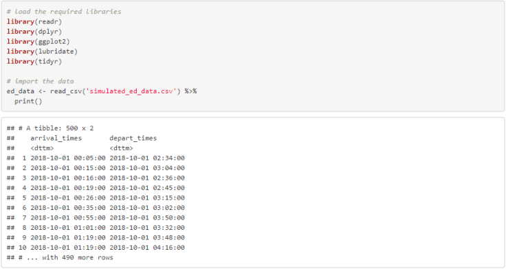
You can access the simulated data in .csv format from this github page, along with all of the code from this example. The data set contains 500 observations with two variables: arrival_times representing arrival times and,  depart_times representing departure times.

Calculating Arrival Volumes

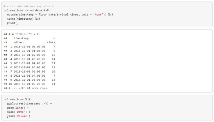
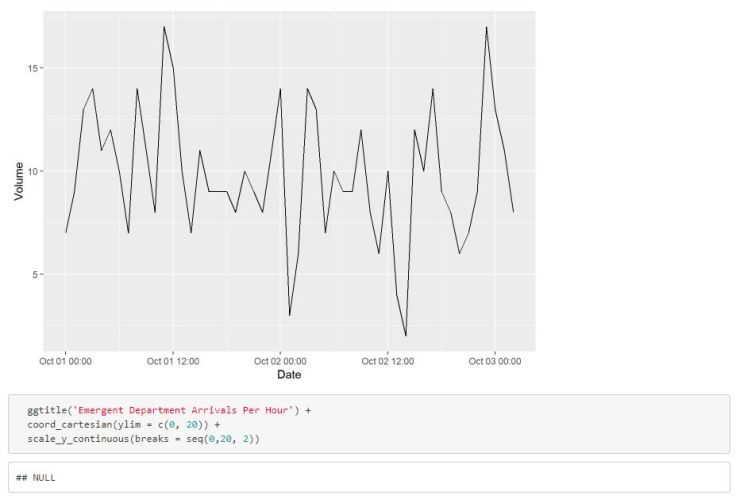
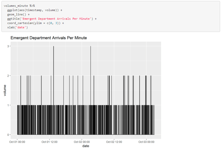
Arrival volumes can be calculated by counting the number of rows of data within a specified time window (hour, day, week, etc…). Functions from the lubridate package make this an especially straight forward task. Below, we will calculate the number of arrivals per hour and plot the results using ggplot. We can use the lubridate::floor_date() function to floor each arrival time to the nearest hour. Then we can simply count the floored timestamp variable.

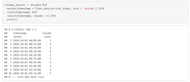
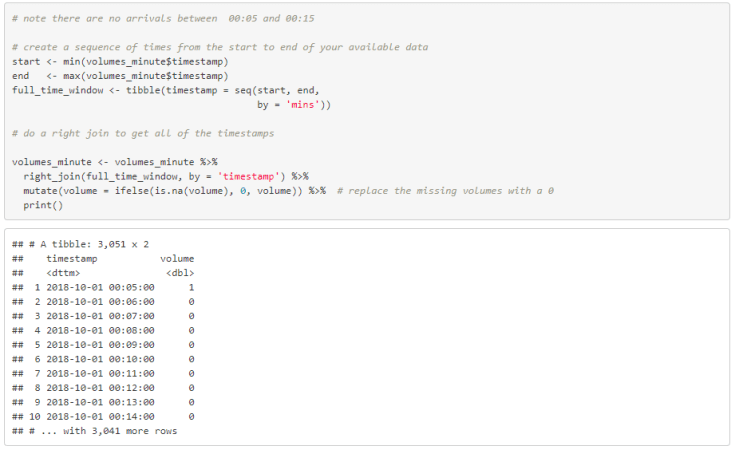
It may be the case that some intervals in your data won’t have any observations (e.g. No arrivals at 2am). In that scenario, you will need to fill in the holes of your time series. The code below shows one solution to this problem for calculating the number of arrivals per minute. You can simply merge your calculated volumes data with another dataset that contains all of the timestamps with the time window of interest.

Calculating Census Volumes

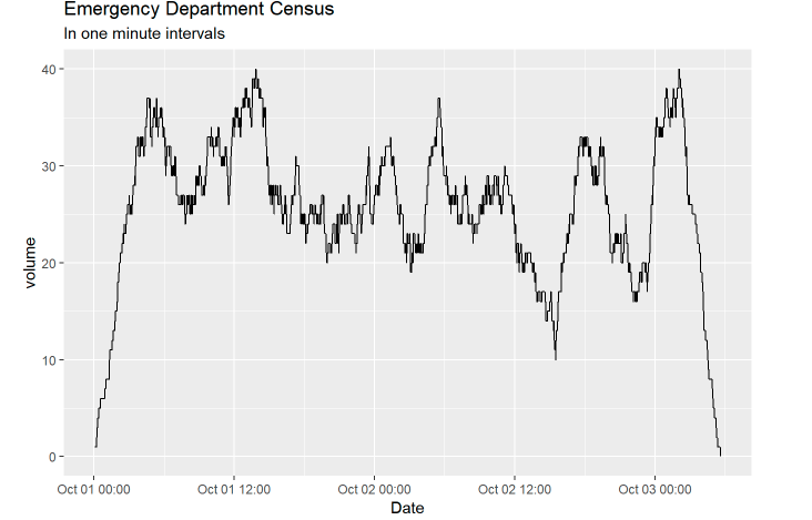
Calculating census volumes, that is the number of patients waiting in the ED at any given time, requires a different strategy. Among the many strategies of accomplishing this, I will focus on one of the faster algorithms.

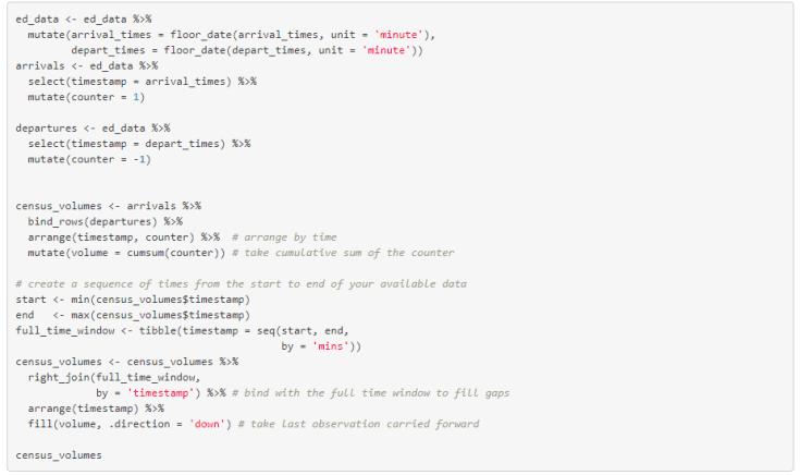
The strategy is to imagine having a counter that keeps track of every time a patient enters or leaves the ED. When a patient walks in the door we add one to the overall count, and when a patient leaves we subtract one. Since we have the timestamps of when patients enter and leave, this is a very simple task.

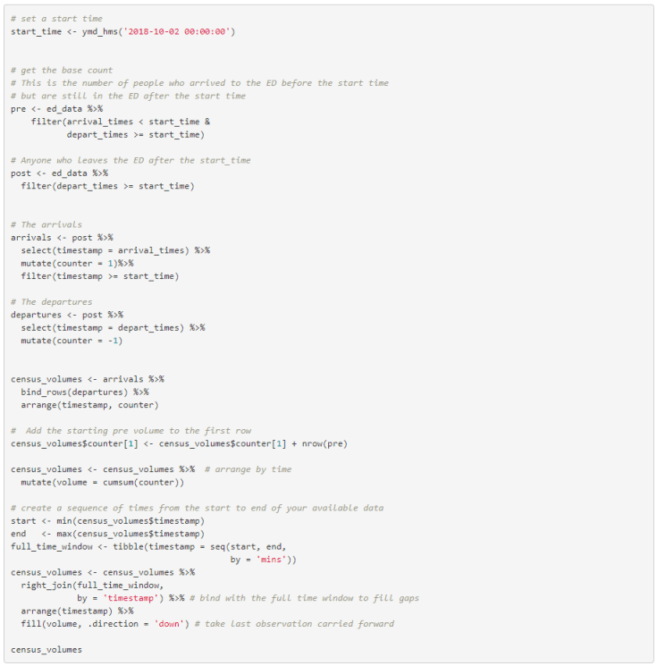
We will split our data into two chunks, one for arrivals and one for departures. For each data split we will create a counter variable. This variable will take the value of 1 for the arrival split and -1 for the departure split. We then bind the two splits back together, arrange them by time, and take a cumulative sum of the counter variable.

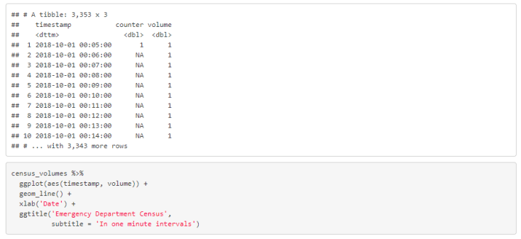
As with the previous example we need to fill in the gaps where no arrivals or departures exist. Except this time, instead of filling in the gaps with zeros we take the last observation carried forward. Since the data will be arranged by time we can use tidyr::fill().

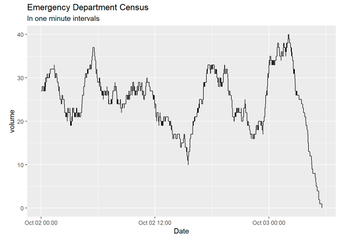
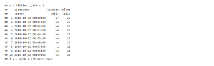
It will rarely be the case where you will be calculating these volumes from scratch, i.e. from the opening of the ED. Let’s redo the above example but take October 2nd at midnight as our starting time.

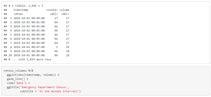
We need to set a start time for our time window. We then calculate the number of people in the ED at the beginning of our time window. We proceed as before, but before taking the cumulative sum we set the first row of the data to be the number of people in the ED at the start time.

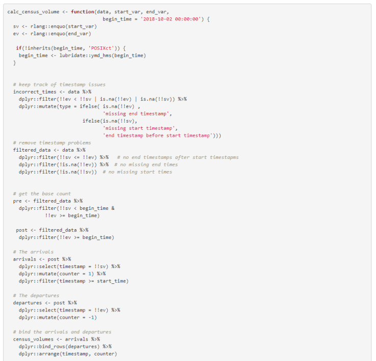
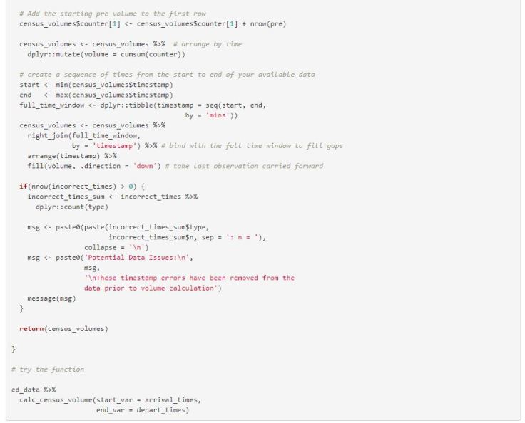
Putting census volume calculation into a function

Since this is a data formatting step that we may run repeatedly, it may be a good idea to create a function to calculate census volumes. The functions handles potential timestamp issues (end times < start times, and missing times). All packages used in the function are explicitly stated using the with :: operator.

Conclusion

The two strategies discussed here can be used for most volume calculations. Before proceeding with either algorithm it is good practice to have a look at your timestamps for accuracy. In using raw timestamp from an Electronic Medical Records system, we may run into some data inconsistencies. It is always a good idea to run some data quality checks before using such data. For example, make sure that there are no departure timestamps that occur before the arrival timestamps.